How to change the tooltip behavior in Tableau for sheets with multiple cards

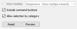
Tableau has two tooltip behaviors

1. Responsive – Show tooltips instantly
2. On Hover – Show tooltips on hover

The default is Responsive. For workbooks published to Tableau Server, I find the behavior On Hover works best with the viz-in-tooltip feature.

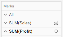
However, changing the tooltip behavior from Responsive to On Hover is complicated if there are multiple cards on the worksheet because Tableau only allows you change the tooltip behavior on the All card which then causes the tooltips to reset on all the other cards.

Sheet with multiple cards

Disabled tooltip setting on SUM(Sales) card

To avoid this it is possible to edit the .twb directly. To change the tooltip behavior for a worksheet called Complex Chart, follow these steps:

1. Backup the .twb in case of errors.
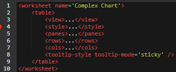
2. Open the .twb in Notepad++ (or another text editor) and search for the worksheet tag with the name attribute set to Complex Chart:
   
3. Collapse the tags until you end up with something like this:
   
4. Before the closing table tag add in a tooltip-style tag with the tooltip-mode attribute set to sticky:
   
5. Save and close the .twb file. Re-open in Tableau and the tooltip behavior for the sheet Complex Chart will now be On Hover.

The tooltip-style tag with the attribute tooltip-mode=’sticky’ is what changes the tooltip behavior to On Hover for all the cards.

Filter on Rank in Tableau

Suppose you have a list of products and you have been asked to display product X and also the 3 products above X and the 2 products below X as ranked by sales. The solution allows the user to enter product X e.g. if the user enters “Milk”:

And if the user enters “Broccoli”:

And if the user enters “Yoghurt”:

The trick is to first create a field called [Rank by Sales] which ranks the products by sales using the formula RANK(SUM([Sales Amount]),’desc’). Then create a field called [Selected Product Rank] which is non-zero only for the selected product using the formula:

IF LOOKUP(MIN([Product]),0) = [p.Selected Product] THEN
    [Rank by Sales]
ELSE
   0
END

The LOOKUP() function allows us to mix the aggregrates ([Rank by Sales]) and non-aggregates ([Product]). Finally create a field called [Filter for 3 above and 2 below] which evaluates to TRUE for the selected product and the 3 products ranked above and the 2 products ranked below the selected product:

(WINDOW_MAX([Selected Product Rank])>4
AND
[Rank by Sales]>=(WINDOW_MAX([Selected Product Rank])-3)
AND
[Rank by Sales]<=(WINDOW_MAX([Selected Product Rank])+2))
OR
(WINDOW_MAX([Selected Product Rank])<=4
AND
[Rank by Sales]<=6)

The expression WINDOW_MAX([Selected Product Rank]) returns the rank of the selected product. Make sure that all the table calculations are computed using Table(Down).